Interactive WebGL Tutorial: Recreating an iOS Animation with GLSL

May 7, 2025

This article explores how to reproduce an iPhone animation I really liked, using WebGL and GLSL shaders. We’ll dive into several foundational concepts in graphics programming: writing simple fragment shaders, leveraging symmetry for shader performance, and compositing with transparency.

Note

Try clicking the animation!

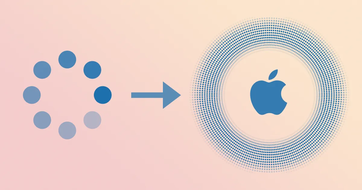
You may have seen this animation in iOS (or iPadOS) if you’ve tried AirPods’ hearing test. It’s made up of thousands of small fading dots, that all expand when touched. Recreating this animation isn’t just fun—it’s also a great way to learn how GPU-based rendering works at a low level using GLSL.

We’ll cover a lot of ground, so buckle up and let’s get started!

Anatomy of an Animation

If you count the individual dots you should land at 3328. That’s a lot of dots. It would be terribly inefficient to draw them one by one, imperative style, for instance creating divs on a page. With WebGL however we can leverage the GPU’s many, many cores and by using a couple of tricks, we’ll make the animation resource usage almost the same whether we’re drawing 5 dots or 3’000 dots.

We’ll start with fewer dots to see what’s happening.

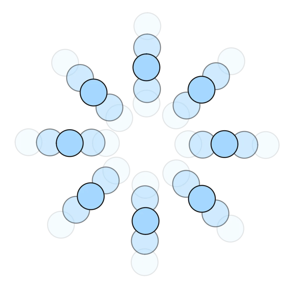
Simplified representation of the Hearing Test animation dots

This simplified representation mirrors the visual style and structure of the iOS original. While simplified, it retains the most important visual characteristics — dot placement, fading, and radial balance.

We’ll first explore how to draw a single dot, then we’ll see how we can create repeated radial patterns (like pizza slices) at no extra computing cost by leveraging its radial symmetry, and finally handle overlapping semi-transparent elements (like a row of dots). As a final touch we’ll make the dots move around.

Drawing a Single Dot

In WebGL, a fragment shader runs once per pixel. Think of each pixel as a mini processor that decides its own color based on a program — though all pixels share the same program, and the only input to the program is the pixel’s position.

Here we will keep things simple and use a single, constant color and we’ll focus on varying the opacity of the pixels.

// Example fragment shader

float get_opacity(vec2 uv) {
    return ... /* opacity definition here */;
}

void main() {
    vec4 rgb = vec4(...) /* known color */;
    vec2 position = ... /* pixel position magically passed in */;
    gl_FragColor = get_opacity(position) * rgb;
}

Note

The shader programs technically run once for every “fragment” and not for every “pixel”. In this article however I’ll use quad-shader — a WebGL helper library I’m writing for this blog — which pretty much maps fragments to pixels. We’ll also assume the pixel position is passed in as an argument to the program when it runs for said pixel — this is also specific to quad-shader.

Since the shader program runs once for every pixel to determine the pixel’s output (opacity here), I find it helpful to imagine the canvas from the perspective of a single pixel — hang with me for a second. So if we are a pixel, and we know our position, how do we go about figuring out our opacity so that — over the whole canvas — a dot is displayed as a result? As mentioned above, only the pixel’s position (which we’ll denote with uv here) is input to the program.

Note

My friend Bas read a preview of this article and pointed me to Conal Elliot’s Functional Images. In a sense, fragment shaders are a way of describing images functionally, where you give a mathematical expression for the image at any position, and the GPU will evaluate it at every pixel!

Let’s assume we want to draw a dot of radius 1.. The most straightforward way is to check if we — the pixel — are at most at distance 1. of the origin.

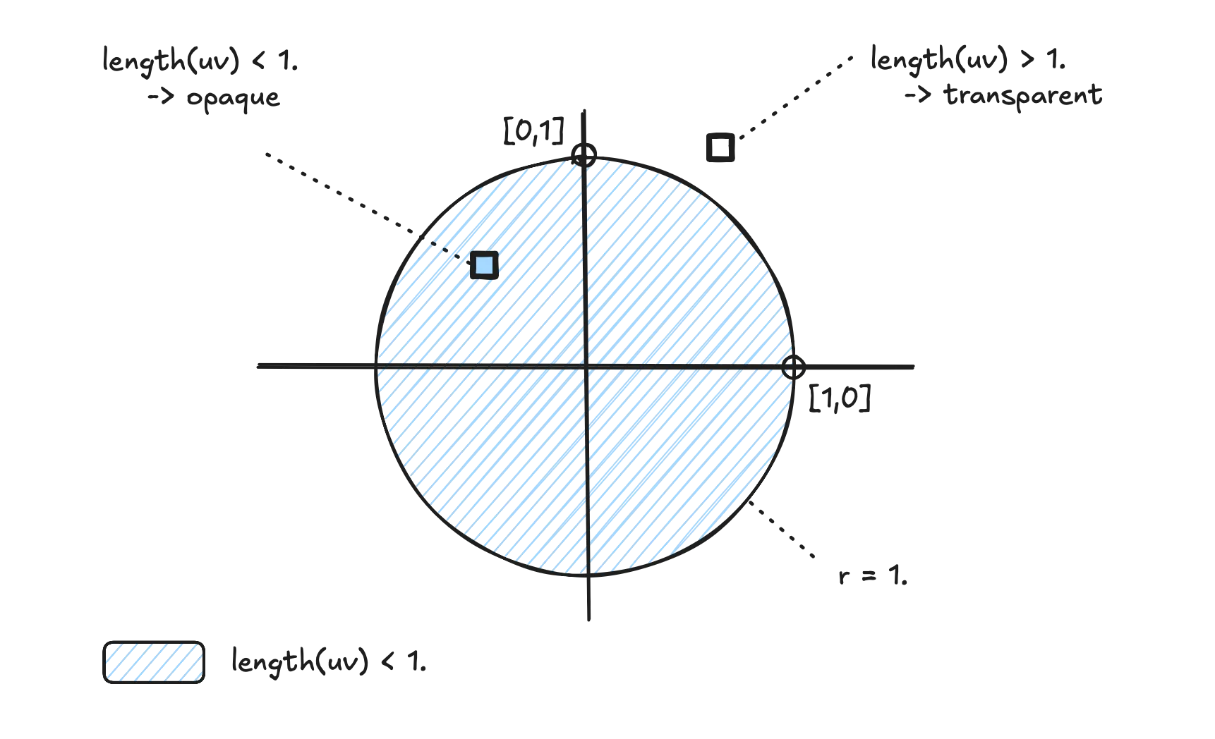
Only pixels within the unit circle will be opaque

If the pixel’s distance to the origin is less than 1., the pixel should be opaque. Otherwise, it should be transparent.

float get_opacity(vec2 uv) {
    if(sqrt(uv.x * uv.x + uv.y * uv.y) < 1.) {
        return 1.; // fully opaque
    } else {
        return 0.; // transparent
    }
}

...

Here we calculate the distance to the pixel from the origin using Pythagoras’ formula of $d = \sqrt{x^2 + y^2}$ and, if $d < 1$, set the pixel to fully opaque (1.) and otherwise fully transparent (0.). This code is very explicit — bordering on verbose. We’ll leverage two built-in GLSL constructs: length() and step().

With length(uv) we get the distance of the pixel to the origin and with 1. - step(1., length(uv)) we get a value that is 1. if inside a circle of radius 1., and 0. otherwise.

If we add in a global input parameter uRadius common to all pixels (unlike uv which is different for each pixel), we can even vary the size of the dot:

return 1. - step(uRadius, length(uv));

Note

step(edge, v) returns 1. if edge < v, and 0. otherwise. Therefore, 1. - step(1., distance) gives 1. when inside the circle and 0. outside. The value of 1. - step(edge, v) is the same as step(v, edge) (arguments swapped) though I find it easier to remember that edge is always the first argument; hence the 1. - ... part.

Note

I’ve created a CodePen where you can experiment with various implementations of get_opacity(). Open index.html and modify get_opacity if you want to follow along.

Try calculating a few values manually if you need to build intuition:

let uv := vec2(0., 0.)
  -> length(uv) =
      sqrt(uv.x*uv.x + uv.y*uv.y) =
      sqrt(0.*0. + 0.*0.) = 0.
  -> length(uv) = 0. -> length(uv) < 1.
  -> step(1., length(uv)) = 0.
  -> get_opacity(uv) = 1. - 0. = 1.
  -> pixel is opaque

Drawing a dot with a given radius was easy enough, let’s now move the dot!

Moving the Dot

By comparing the length of the position vector (distance from origin to the pixel) to the radius, we were able to draw a dot centered at the origin. What if we wanted to draw a dot not at the origin, but centered at some other position $c$? Let’s imagine we want to draw a dot to the right of the origin. Instead of directly calculating whether length(uv) is smaller than the radius, we shift the pixel’s position by subtracting $c$, effectively centering our calculations at c instead of the origin:

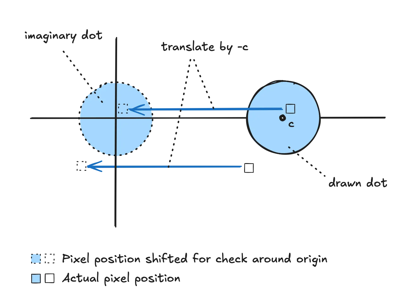
Two of the many pixels rendering a dot (disc) of radius r centered at c

So we run the same calculation as above to check whether we are inside a unit circle, but on modified coordinates, and not directly on the pixel’s position.

return 1. - step(uRadius, length(uv - vec2(uShift, 0.)));

This is the name of the game when doing shady shader stuff: find a way to describe a shape mathematically around the origin; then in order to move it we “shift the canvas” by subtracting the actual center before performing the check. If you ever need to draw shapes more complex than dots (and I hope you do!), see Inigo Quilez’s 2D distance functions which describe many more shapes like rounded boxes, triangles, stars, etc.

Repeating Patterns for Free with Modulo

Now that we can draw one dot and position it wherever we want, let’s see how we can draw multiple dots. For our animations, we can take advantage of the fact that it’s radially symmetrical. We’ll see that by using the mod() (modulo) operator on the parameters that describe a pattern, we can make the pattern repeat without having to resort to e.g. loops. This will basically repeat the pattern multiple times at no extra (GPU) cost.

In order to simplify things we will work with polar coordinates. Quick refresher, this coordinate system lets us express the position $(x, y)$ in terms of $\rho$ (or rho) and $\theta$ (or theta), where $\rho$ is the distance to the origin and $\theta$ the so-called “polar angle”.

$\rho = \sqrt{x^2 + y^2}, \theta = arctan(y,x)$

In GLSL we can use the following primitives to convert uv to polar coordinates:

float theta = atan(uv.y, uv.x)
float rho = length(uv)

As mentioned above, the trick is to define a general pattern in terms of a parameter (we’ll use $\theta$), and then by using the modulo operator, we can make the pattern repeat at will.

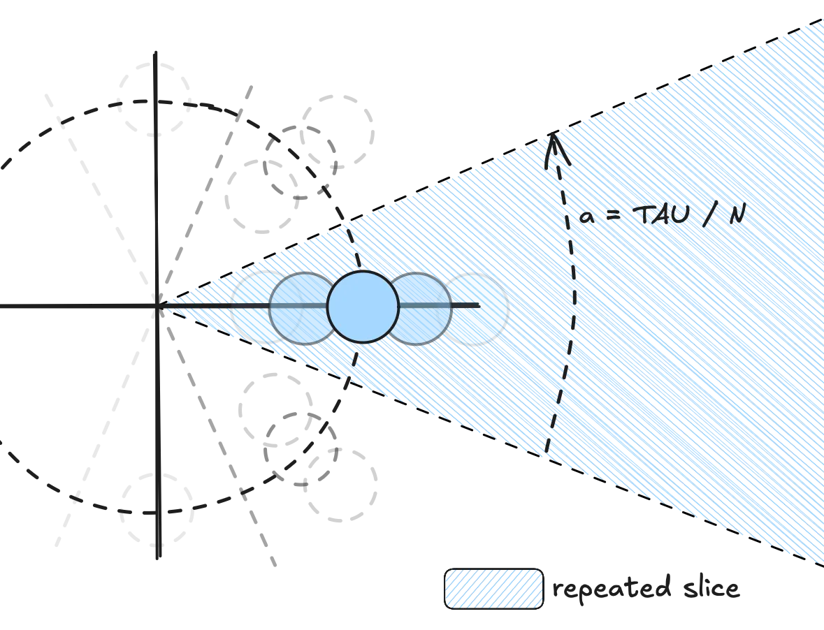
The slice that is described once and repeated N times

Note

To simplify calculations we work with $\tau = 2 \pi$, referred to as TAU in the code. There’s lots of good reasons for using $\tau$ instead of the very famous $\pi$. In particular here it will come in handy to have $\tau$ represent a full rotation in radians (around the unit circle).

Let’s start simple and say we want to repeat a gradient (we’ll get to the dots in a minute) radially N times and have the opacity follow $\theta$. If we make the opacity grow with $\theta$ for pixels in $0 \leq \theta < \tau/N$ we would get a nice radial gradient. By slapping the mod operator on top, as soon as $\theta$ goes beyond $\tau/N$ again, the gradient will repeat — and create $N$ slices with the repeating pattern.

Using this we can repeat the pattern any number of times with constant time — technically $O(1)$ w.r.t to the number of symmetries or repeated “slices”.

float a = TAU/uSymmetries; // the size (angle) of each slice

float theta = atan(uv.y, uv.x); // returns the pixel's angular position within [-TAU, TAU]

return mod(theta, a) / a; // loop angular position between 0 and 'a' and scale betwee 0 and 1

This means that, as long as we can describe a pattern in terms of theta and rho, we can repeat that pattern radially as many times as we want without any extra resource usage.

Radially Repeating Dots

Gradients are pretty, but we’re here to draw dots. We can use the same trick to make $\theta$ repeat, and we can adapt the checks from the first section to figure out if the pixel lands in a dot.

float radius = .2;

float a = TAU/uSymmetries;
float a2 = a/2.;

/* switch to polar */
float theta = atan(uv.y, uv.x); // between -TAU/2 and TAU/2
float rho = length(uv);

/* shift theta to align the center of slice 0 with the X axis */
theta += a2;

/* atan() returns a value from [-TAU/2, TAU/2] and for simplificy when calculating
 * indices below we move it to [0, TAU] which is equivalent */
theta = mod(theta + TAU, TAU);

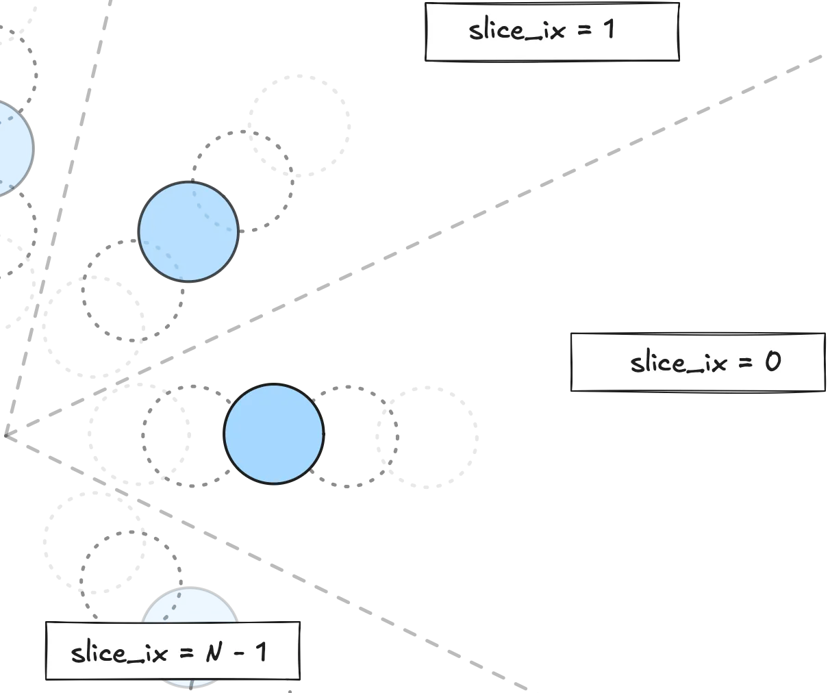
/* index the slices with slice 0 around theta == 0*a, slice 1 around theta == 1*a, etc */
float slice_ix = floor(theta / a);
theta = mod(theta, a); /* make everything repeat between [0, a] */

theta -= a2; /* compensate for shift above */
uv = vec2(rho*cos(theta), rho*sin(theta)); /* back to cartesian */

float opacity = 1. - step(radius, length(uv - vec2(.8, 0.))); /* dot shifted to the right */
opacity *= (1. - .8 * slice_ix / uSymmetries); /* vary opacity depending on the slice */

return opacity;

One added thing here is slice_ix, which is the index of the slice the current pixel is in. This is useful if you want to vary a parameter based on which slice you’re in (if you just used theta instead of slice_ix the value would vary within the same slice, try it out in the CodePen). This is used in this snippet to give each dot a different opacity.

Each dot/slice has a different opacity

Now that we’ve established how to repeat patterns radially around the center, the next logical step is to build more structure within each slice. After all, the original animation doesn’t just have one dot per slice — it has rows of them, extending out. To recreate this, we’ll need to position multiple dots along the direction of each radial slice — though we’ll only need to describe it once, along the horizontal axis.

Repeating Dots Horizontally

Let’s consider the slice with index 0, extending along the horizontal axis towards (plus) infinity. We’ll have several dots, each at distance $d$ (uDist in the code) from each other, potentially overlapping:

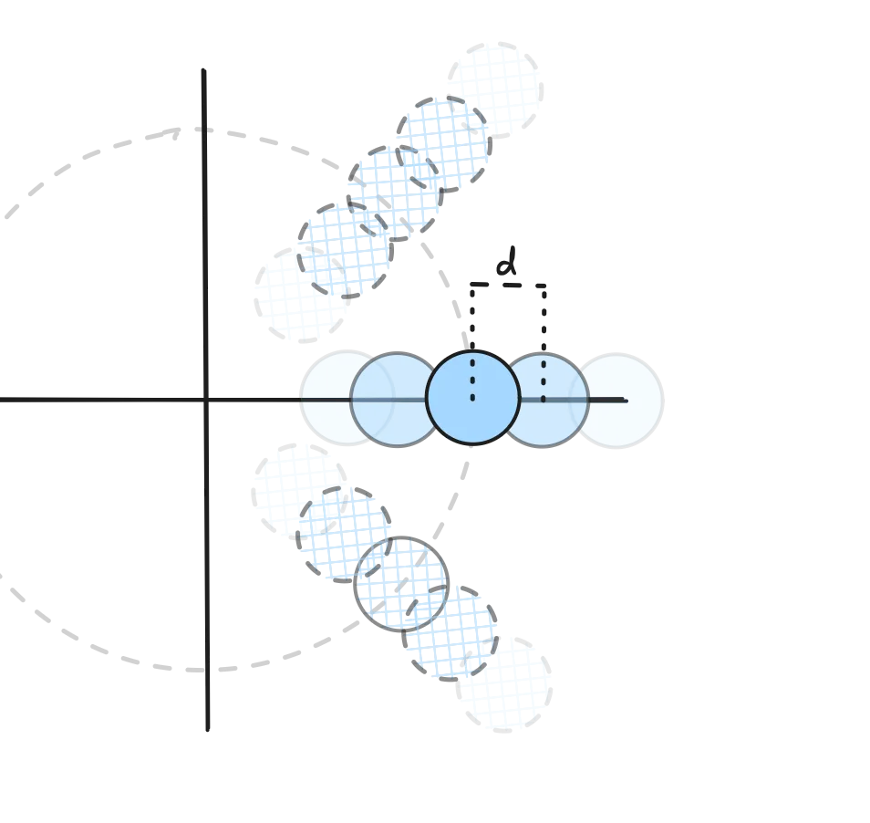
Dots separated by distance d

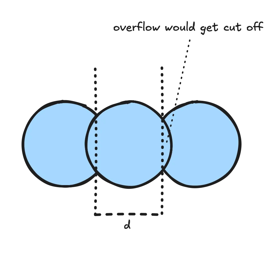
We saw earlier that we could leverage the modulo operator to repeat patterns. This mod trick can be used for other parameters, for instance x if we want linear symmetries instead of radial symmetries. But we run into an issue.

Can you spot it?

const float radius = .3;
float uDist2 = uDist/2.;

/* number of dots on the left and right of the center dot */
const int nSideDots = 1;

/* get index (use absolute value to mirror around 0) */
float dot_ix = abs(floor((uv.x + uDist2)/uDist));
uv.x = mod(uv.x + uDist2, uDist) - uDist2; /* repeat every 'uDist' */

/* Return 0. (transparent) _if) uv is now _outside_ of the dot at the origin
    _or_ unless if the index is greater than the number of dots to draw. */
return (1. - step(radius, length(uv))) * 1. - step(float(nSideDots + 1), dot_ix);

You guessed it (or not): the pattern repeats exactly — and the dots don’t blend together; moreover the overflows are hidden. The same limitation applies to $\theta$, but as long as dots don’t cross slice boundaries, it’s imperceptible — our little secret.

Here unfortunately there is no way to do this in constant time, like with the radial repetitions. While there would be workarounds if we had overlapping opaque discs, there is no workaround for handling transparency — which is used in the original iOS animation. To solve this issue we need to calculate the opacity at every point, taking all other (potentially overlapping) discs into account.

Compositing Overlapping Dots

If two overlapping dots have opacity .5 we may be tempted to multiply the individual opacities to get the overlap’s opacity, though a quick example shows that this won’t work: if the dots have opacity .5, the resulting opacity should come out greater than the individual opacities, though if we do the math with the naive technique we get the following: $0.5 \cdot 0.5 = 0.25 < 0.5$.

We also run into an issue if we add up the opacities: two dots with an opacity of .5 each would make for an opacity of 1. already (fully opaque) and we know that’s not how things work “in the real world”. Adding a third dot, the opacity would go up to 1.5 or $150\%$ (whatever that might mean) so clearly this technique doesn’t work either.

To get an idea of how we’ll solve this, let’s look at the real world — though we are modeling a virtual animation, our visual expectations do come from experiences “IRL”.

Let’s assume we have three sheets of the same material which is slightly opaque, and let’s say each sheet lets 20% of the light through and blocks the remaining 80% of the light. We’ll say each sheet is 80% opaque — this might not be scientifically precise, but it serves as a helpful mental model. Now let’s picture a photon (light particle) that has to go through all three sheets of the material.

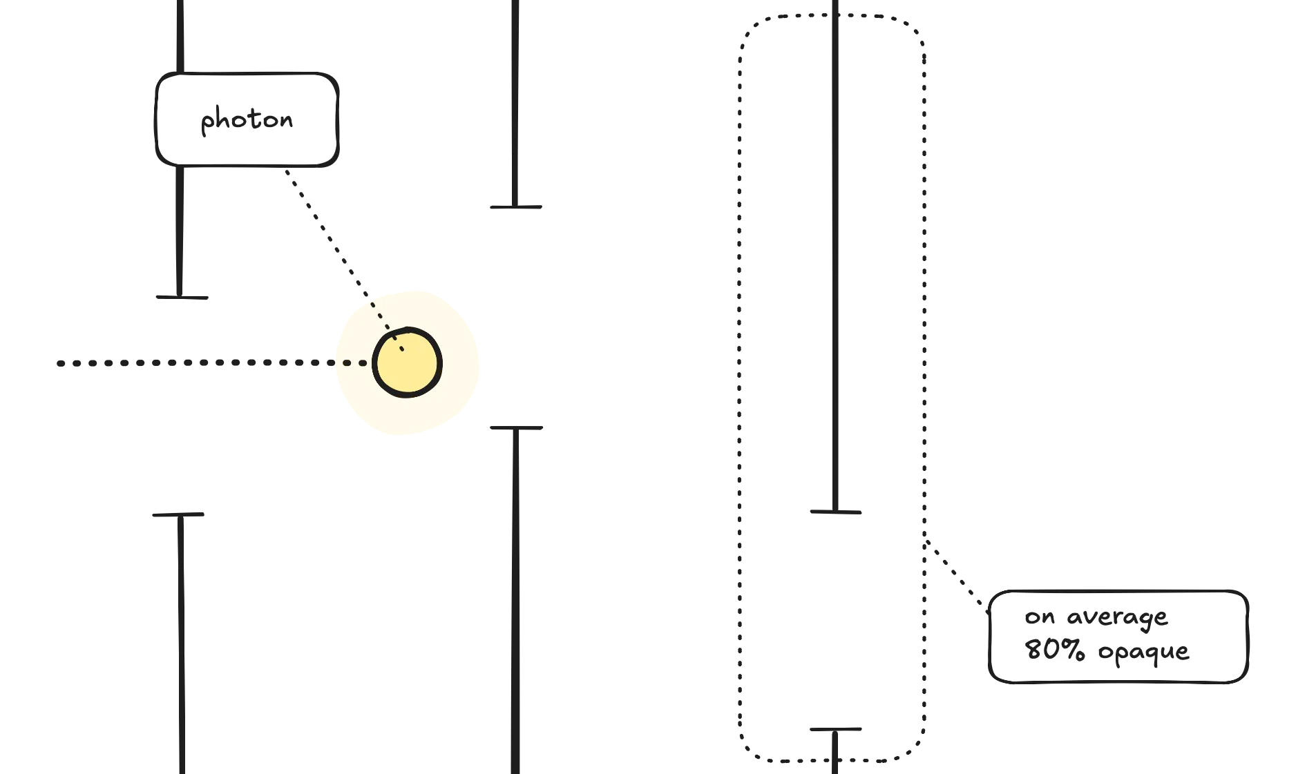
Photon going through sheets of material

Wave-particle duality notwithstanding, what is the probability that the photon will manage to go through all three sheets? If one sheet of material — on average — blocks 80% of the light, let’s say that the photon has 20% chance of going through the first sheet; in other words the probability is $0.2$. The probability of the photon going through both the first sheet and the second sheet would then be $0.2 \cdot 0.2 = 0.04$ and finally for three sheets the probability would be $0.2^3 = 0.008$. The probability that the photon will hit any of the three sheets is then $1 - 0.008 = 0.992$, meaning the resulting opacity is 99.2% (for this definition of opacity).

Using the “transparency” (or one minus the opacity) for the sheets allowed us to multiply the individual tranparency values. Let’s say in general transparency is $t = 1 - o$ where $o$ is the opacity. Let’s say all the different layers have transparency $t_0, t_1, ...$. Following the 3-sheet-photon idea above, we can calculate the total opacity as one minus the product of the transparencies, or:

$o = 1 - t = 1 - (t_0 \cdot t_1 \cdot ...) \\ = 1 - \prod t_i \\ = 1 - \prod (1 - o_i)$

The implementation would look something like this:

float radius = .3;

/* how many dots to the side (right, left) of central dot */
const int nSideDots = 1;

float product = 1.; /* current product result */

for (int i = -nSideDots; i <= nSideDots; i ++) {
    float opacity = .5; /* any dot's opacity */
    vec2 shift = vec2(float(i)*uDist, 0.); /* position over dot */
    opacity *= 1. - step(radius, length(uv + shift)); /* only consider current dot */
    product *= (1. - opacity);
}

return 1. - product;

Note that this operation is commutative, so it doesn’t matter what order we look at the dots — though this would be different if we were mixing colors as well.

Note

There’s actually a whole world of alpha blending and compositing techniques out there, and I’m just scratching the surface here. What I’ve described is one way to think about it, but if you want to go deeper (or catch mistakes I’m probably making here), the Wikipedia article on alpha compositing is a great starting point. It covers more formal models and edge cases I’m probably hand-waving past.

One caveat: GLSL in WebGL has limited support for dynamic control flow. For example (very much simplifying here) you can’t loop over an arbitrary number of dots or slices unless the loop bounds are known at compile time — hence why nSideDots is a const. This constraint can shape how your compositing logic is structured; here for instance we set the number of dots as a compile-time constant.

Final Result & Conclusion

Alright, so we’ve drawn a dot, made it move, repeated it in slices, stacked those repeated dots with overlapping transparency, and somehow survived all the shader math (I hope? Let me know!). Time to put it all together and see what this looks like — and let’s add a bit of motion.

float radius = .1;

float a = TAU/uSymmetries;
float a2 = a/2.;

/* switch to polar */
float theta = atan(uv.y, uv.x); // between -TAU/2 and TAU/2
float rho = length(uv);

/* shift theta to align the center of slice 0 with the X axis */
theta += a2;

/* atan() returns a value from [-TAU/2, TAU/2] and for simplicity when calculating
 * indices below we move it to [0, TAU] which is equivalent */
theta = mod(theta + TAU, TAU);

/* index the slices with slice 0 around theta == 0*a, slice 1 around theta == 1*a, etc */
float slice_ix = floor(theta / a);
theta = mod(theta, a); /* make everything repeat between [0, a] */

theta -= a2; /* compensate for shift above */
uv = vec2(rho*cos(theta), rho*sin(theta)); /* back to cartesian */
uv.x -= .5;

/* how many dots to the side (right, left) of central dot */
const int nSideDots = 1;

float product = 1.; /* current product result */

float period = 5.; /* period of 2 seconds */
float dist = uDist + uDist/5. * sin(TAU/period * uTime + slice_ix);

for (int i = -nSideDots; i <= nSideDots; i ++) {
    float opacity = .5; /* any dot's opacity */
    vec2 shift = vec2(float(i)*dist, 0.); /* position over dot */
    opacity *= 1. - step(radius, length(uv + shift)); /* only consider current dot */
    product *= 1. - opacity;
}

return 1. - product;

Handling user interactions like clicks (as in the very first animation) is left as an exercise to the reader (see here for the first animation’s source). And while you’re at it, why not play with the colors a bit too!?

Fell in love with iPhone's "Hearing Test" animation, just had to try and recreate it #generative #art

[image or embed]

— Nicolas Mattia (@nmattia.bsky.social) 12 April 2025 at 22:38

Let me know if you enjoyed this article! You can also subscribe to receive updates.

Here's more on the topic of WebGL and JavaScript:

• SKÅPA, a parametric 3D printing app like an IKEA manual
• How to Set WebGL Shader Colors with CSS and JavaScript